What We Know

The measurements of the “solar” and “atmospheric” oscillation parameters are now becoming quite precise (see figures 15 and 16), which means that we have to consider the full three-flavour oscillation analysis instead of assuming that only two flavours mix in any given experiment. Three flavours correspond to a three-dimensional rotation, which involves three angles (roll, pitch and yaw in the terminology of aircraft and boats), three mass differences (one of them being the sum of the other two), and one phase. The phase is the only difference between neutrino mixing and “real” rotations: it is only present if all three flavours mix, and it has a different sign for neutrinos and antineutrinos (in the terminology of particle physics, it is CP violating). This is potentially very important: one of the greatest mysteries of modern cosmology (along with dark matter and dark energy) is why the universe appears to be made up of matter, and not a 50:50 mixture of matter and antimatter, despite the fact that particles and antiparticles are usually created as particle-antiparticle pairs and have nearly identical interactions. CP-violating processes hold the key to solving this mystery.

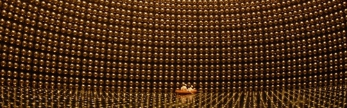
The relationship between the three neutrino mass states (ν₁, ν₂, ν₃) and the three flavour states (ν_e, ν_μ, ν_τ) is usually expressed as a 3×3 matrix known as the PMNS matrix after Bruno Pontecorvo, Ziro Maki, Masami Nakagawa and Shoichi Sakata. This can be written in terms of the three mixing angles and one phase in the form

where s₁₂ = sin(θ₁₂), c₁₂ = cos(θ₁₂), δ is the CP-violating phase, and the extra phases α_1,2 only come into play in double-beta decay.

The key features of this rather forbidding-looking object are as follows:

• The angles θ₁₂ (solar neutrino oscillation) and θ₂₃ (atmospheric neutrino oscillation) are fairly well determined, and are large (θ₁₂ = 33.4°±0.8° and θ₂₃ = 49°±1°, though the first-octant value of 41° is still possible at lower probability).
  • This is unexpected: in the equivalent mixing matrix for quarks (the Cabibbo-Kobayashi-Maskawa or CKM matrix) all the angles are quite small, and the 3×3 matrix is nearly diagonal.
• The third angle θ₁₃, unlike the other two, is quite small, but has now been quite precisely measured thanks to the work of T2K, NOνA and the reactor antineutrino disappearance experiments Daya Bay and RENO. A recent global fit gives θ₁₃ = 8.6°±0.1°.
  • A non-zero value of θ₁₃ is necessary to observe the CP-violating phase δ.
  • There are currently strong hints that δ is non-zero – the 3σ range preferred by the global fits no longer includes the entire range of possible values – but nothing approaching the 5σ threshold that particle physicists require for a discovery.
    

Because Δm₁₂² << Δm₂₃², the difference between Δm₂₃² and Δm₁₃² is small, regardless of which hierarchy is correct. This means that a value of L/E appropriate to maximise the effect of θ₁₃ will also be appropriate for θ₂₃, which is much larger. As the atmospheric neutrino oscillation is known to involve muon-neutrinos and not electron-neutrinos, this is principally a problem for accelerator-based neutrino oscillation experiments such as T2K and MINOS. Reactor-based experiments have an electron-antineutrino beam, so the relevant mass splittings Δm₁₂² and Δm₂₃² are well separated and L/E can be tuned to pick out one or the other.

Basics of Oscillation Experiments

Neutrino oscillation experiments are designed specifically to study changes in neutrino flavour – unlike the experiments that actually discovered the effect, which were just designed to detect neutrinos. There are two basic strategies:

• disappearance experiments, in which you know how many neutrinos of a specified type you produce, and you count the number of that same type of neutrinos that you detect at distance L – the oscillation signal is a deficit in the number observed;
• appearance experiments, in which you produce neutrinos of one type but observe neutrinos of a different type – the signal is the observation of a non-zero number of this different type (after allowing for any backgrounds).

Reactor neutrino experiments are always disappearance experiments, because the energies of reactor neutrinos – typically a few MeV – are not sufficient to create muons or taus, and therefore ν_μ and ν_τ cannot be seen in charged-current reactions. The only way to do an “appearance” experiment with low-energy neutrinos is direct comparison between neutral-current and charged-current reactions, as in the solar-neutrino experiment SNO. Although this was a beautiful experiment, it relied on the availability of large quantities of heavy water, which is not in general practical (SNO was a special case), so disappearance is the only realistic option.

The key issue with disappearance experiments is an accurate understanding of two things: your incoming neutrino flux (obviously, to work out how many have disappeared you need to know how many you expected in the first place) and the efficiency with which you detect events (if you are over-optimistic about this, you may think neutrinos have disappeared when in fact they were there but you missed them). The calculation of reactor fluxes is quite challenging (see our earlier discussion of artificial neutrino sources), so this has in fact been the limiting factor in some reactor experiments. If your experiment is designed to study neutrinos from one specific reactor, like Chooz, you can monitor the incoming flux by constructing two similar detectors, one close to the reactor (measuring the neutrinos before they have a chance to oscillate) and one further away: taking the ratio of the signals cancels out both the overall flux and – if the near and far detectors are of the same design – much of the uncertainty in detector efficiency. This is not so easy if, like KamLAND, you detect the combined flux from many reactors. In this case, a near detector is not really practical, although you can make some checks (if your statistics are high enough) by correlating changes in the observed flux with recorded changes in the power output of the reactors.

As reactor neutrinos have quite a large energy spread, a detector at a given distance L is actually recording events at a range of values of the combination L/E which actually occurs in the oscillation equations. This means that, if your detector has good energy resolution, you can check that you are really seeing oscillation by looking for the expected sin²(1.267 Δm² L/E) behaviour. Figure 18 shows such a plot made by the KamLAND experiment. This is an important check that the signal really is from oscillation: if it were caused by an error in the calculated flux, or by unsuspected problems in reconstructing the events, you would not expect to see this nice sinusoidal pattern.

Appearance experiments could be said to be more elegant than disappearance experiments, in that there can be no arguing with a positive result: if your initial beam was pure type X, and you see some neutrinos of type Y, something has definitely happened. In practice, the distinction is not so clear-cut: accelerator-generated muon-neutrino beams are not 100% pure (they always contain a small fraction of electron-neutrinos), and particle identification in detectors is not 100% efficient (there is a chance that you see an event of type X, but mistake it for type Y, or that you see an event which is simply background, neither X nor Y, but identify it as type Y). This sets up the key design issues for appearance experiments: you must have a good understanding of your beam, including an accurate estimate of the intrinsic contamination from other flavours, and you must have a very well-understood detector, with good particle identification, and a good knowledge of any possible background processes.

Beam characterisation requires a near detector: you measure the beam before it has a chance to oscillate, and compare these results with the results from your far detector. If the near and far detectors are very similar (the near detector perhaps scaled down to reflect the higher flux), comparing near and far detectors will also cancel out some detector effects, as with the disappearance experiments. This is the approach taken by the MINOS experiment – which is primarily a disappearance experiment, but is also designed to look for ν_e appearance.

In T2K, the near detector is also tasked with improving our understanding of possible background processes, by making measurements of various types of neutrino interaction for which the current world data sample isn’t very good. An important example is the production of neutral pions, π⁰s, in neutral-current interactions, ν_μ + p/n → ν_μ + p/n + π⁰. The π⁰ decays into two photons. Photons in water Cherenkovs look almost identical to electrons, so if one of the photons is missed because it happens to have very low energy, you have an event that could easily be mistaken for an electron-neutrino charged-current interaction. For this reason, and because the detector is located so close to the accelerator that the number of events is expected to be large, the T2K near detector ND280 is not a water Cherenkov detector but a tracking detector. The advantages of this approach are expected to outweigh the disadvantages of having different efficiency calculations for near and far detectors.

In practice, appearance experiments using an accelerator-generated muon-neutrino beam are always disappearance experiments as well: because Δm₂₃² and Δm₁₃² are so very similar, an experiment designed to look for ν_e appearance (θ₁₃) will also be sensitive to ν_μ disappearance, and the detector design needed for the appearance experiment (a near detector to measure intrinsic contamination of the beam, good electron-muon separation, good background rejection) is also very suited to disappearance measurements (the near detector gives you the muon-neutrino flux before oscillation, and the good particle identification and good background rejection are also useful for the disappearance analysis).

Example disappearance experiments: Double Chooz (reactor experiment, successor to Chooz); KamLAND.

Example appearance experiments: MINOS, T2K, OPERA (tau-neutrino appearance), ICARUS (multi-purpose liquid argon tracking detector), MiniBooNE.

Three-Neutrino Oscillations

The NuFIT group provide a regularly updated global fit to neutrino oscillation data, with values of the mixing angles, the two independent squared mass differences, and the elements of the PMNS matrix. As of summer 2021, the most recent update (July 2020) gives good constraints on everything except δ, which still has a very wide 3σ range (though there is now a preference for values around 200° for normal ordering, m₁ < m₂ < m₃, and around 300° for inverted ordering, m₃ < m₁ < m₂).

In the “nearly Standard Model” picture of three neutrinos with small but non-zero masses and large mixing between flavours, this is the current state of the art. It raises interesting questions: we have no idea why θ₁₂ and θ₂₃ are so large compared to θ₁₃ (and compared to the mixing angles in the quark sector of the Standard Model), we don’t know which hierarchy is correct, we know very little about δ (although, with θ₁₃ larger than we thought it might be, we have a good chance of measuring this in the next generation of oscillation experiments), and we don’t know whether the neutrino and the antineutrino are the same particle or not. If this were the whole story, neutrino physics would be an interesting field for years to come. However, some results not included in this fit may prove to herald yet more surprises in the story of neutrinos.

Beyond three-flavour oscillations: LSND, MiniBooNE and the mystery of the fourth mass

The Standard Model has three of everything: three charge +2/3 quarks; three charge –1/3 quarks; three charged leptons; three neutrinos. It is, of course, possible that a fourth generation of quarks and leptons could exist, if it were too massive to be detected in current accelerators. However, we do definitely know that there is no fourth light neutrino, so if there is a fourth generation, it has a neutrino that is very unlike the three we know about.

With three neutrinos, there are only two independent mass differences: the third difference has to be the sum of the other two (if Joe is 2 years older than Alice, and Alice is 3 years older than Kim, we know Joe is 5 years older than Kim). Since the solar and atmospheric neutrino oscillations yield very distinct mass differences, we have accounted for all three neutrinos in the oscillation measurements discussed above.

Unfortunately, for some years there has been an unexplained result from another oscillation experiment: LSND, a short baseline (L = 30 m) oscillation experiment looking at ν_μ → ν_e, with the ν_μ produced by the decay of pions at rest (not in flight as is usual for accelerator-generated neutrino beams). The decay of π⁺ at rest produces a μ⁺ and a ν_μ, and the subsequent decay of the muon (which is also very nearly at rest) produces a ν_e and a ν_μ. Therefore, although the neutrinos produced are a mixture of electron and muon type, the antineutrinos are pure muon-type: looking for inverse beta decay, ν_e + p → e⁺ + n, is thus a sensitive appearance experiment for electron-antineutrinos. Even with a low-energy beam, the short baseline means that LSND has a rather small value of L/E, and so is sensitive to much higher values of Δm² than those observed in solar and atmospheric oscillations. Nevertheless, this experiment observed a large excess of inverse beta decays over the calculated background, consistent with a signal from a squared mass difference of 0.05–100 eV², which is quite inconsistent with the solar and atmospheric squared mass differences given by three-flavour analyses.

Another experiment using neutrinos from pion decay at rest, KARMEN, found no evidence for neutrino oscillations. As the baseline of the KARMEN experiment (17 m) is slightly shorter, this null result does not completely contradict the LSND result, though it does reduce the allowable range of Δm² to 0.05–1 eV² (still inconsistent with the solar and atmospheric results), or 0.2–1 eV² when constraints from other short-baseline experiments were taken into account. When these results were first announced around the turn of the millennium, the general reaction of the neutrino physics community was that one anomalous result was not enough evidence on which to base a major revision of the Standard Model, so over the next decade there was a general tendency to ignore the LSND result as probably wrong (presumably owing to some unsuspected additional background source). This tendency was strengthened in 2007 when the MiniBooNE experiment, a conventional accelerator neutrino experiment with L/E designed to explore the LSND signal region, found no evidence for ν_μ → ν_e oscillations (see figure 19).

MiniBooNE was using neutrinos, whereas LSND and KARMEN were sensitive to antineutrinos. To remove this slight difference, MiniBooNE subsequently took data with an antineutrino beam (generating by setting the focusing horns in the beampipe to select π^– instead of π⁺). To everyone’s great surprise, these data did show an excess, with large error bars because of comparatively low statistics, but completely consistent with the original LSND result. Taken at face value, this indicates:

• there is an oscillation signal corresponding to mixing between ν_μ and ν_e with a squared mass difference of about 0.2–1 eV² and a mixing angle of 0.001 < sin² 2θ < 0.03;
• neutrinos behave differently from antineutrinos, which show no such oscillation.

In addition, the MiniBooNE neutrino data showed an excess of electron-like events at low energies, inconsistent with the LSND signal and indeed inconsistent with any oscillation picture, but not explained by known backgrounds. The statistics for the antineutrino data are not sufficient to confirm or refute a similar excess in the antineutrino data.

While it is clear that more statistics are needed to confirm the excess, the apparent agreement of MiniBooNE and LSND in the antineutrino sector does suggest that something is going on, and that something cannot be incorporated into the standard three-neutrino model. So why are we sure that a fourth neutrino similar to the three we know about is not the answer, and what other possibilities exist?

Counting neutrinos

Neutrinos interact by the weak interaction, and that means that the carriers of the weak force, the W^± and Z bosons, can decay into neutrinos: specifically, W⁺ → l⁺ + ν_l (where l = e, μ or τ), W^– → l^– + ν_l, and Z → ν_l + ν_l. The more distinct types of neutrino there are, the more ways the W and Z can decay, and therefore the shorter their average lifetime. In quantum mechanics, the Uncertainty Principle relates time to energy, and therefore a particle’s lifetime to its mass: the shorter the lifetime, the greater the uncertainty in the mass (known as the width). Hence, if we measure the width of the Z boson, we can determine how many different types of neutrino it can decay into. This was done at the LEP Collider at CERN, the predecessor of the LHC. LEP collided electrons and positrons: since the Z can decay into e⁺e^–, if you arrange for the total energy of the electron and positron beams to be equal to m_Zc², a collider like LEP will make large numbers of Z bosons, and can therefore measure the width of the Z with great precision. The result is shown in figure 20: the data agree well with 3 neutrino species, and rule out 2 or 4 convincingly. Therefore we conclude that, if there is a fourth generation of Standard Model matter particles too heavy to be discovered in current experiments, it cannot have a neutrino light enough to be produced in Z decays. It certainly can’t have a neutrino light enough to account for the LSND/MiniBooNE oscillation signal.

Sterile neutrinos

So, we need four neutrinos to account for three distinct and unrelated squared mass differences, but we can’t have four Standard Model neutrinos because the Z width won’t permit it. Does this mean that the LSND result has to be wrong?

The answer is no, because the Z width experiment counts only neutrinos that the Z can decay into. If there exist neutrinos that do not feel the weak interaction – for example, right-handed neutrinos – they would not be included in the Z width count, but they might still mix with the three known neutrinos. Such particles are called sterile neutrinos.

Although the original formulation of the Standard Model called for massless neutrinos, it could be argued that including neutrino masses simply puts neutrinos on the same footing as the other Standard Model particles, and therefore isn’t really “beyond the Standard Model” physics.  However, sterile neutrinos definitely are “beyond the Standard Model”, and therefore there are no predictions of their properties or behaviour available. All we can do is to use existing data to infer the properties that such particles would need, and try to design future experiments to test for this.

Evidence in favour of sterile neutrinos

• The LSND and MiniBooNE antineutrino data.
• Possibly, reactor neutrino data in general. Recent recalculations of the reactor antineutrino flux suggest that it ought to be 3% larger than previously thought. If this is true, all the reactor neutrino experiments that agreed with previous calculations of the reactor flux were actually measuring a small deficit, which might be accounted for by oscillation into sterile neutrinos.
• Results from big bang nucleosynthesis, i.e. the production of the light isotopes ²H, ³He, ⁴He and ⁷Li in the early universe, a few minutes after the Big Bang. Calculations, e.g. [11], slightly favour four neutrino species, although not significantly: the fitted value is N_ν = 3.71±0.46. This result does at least disfavour more than 4 neutrinos (not trivial, as theorists often introduce two sterile neutrinos in an attempt to deal with the discordances in the oscillation data).
• Possibly, the low energy excess in the MiniBooNE neutrino data (it doesn’t look like an oscillation signal, but if a sterile neutrino model were to provide an explanation of it, that would certainly be a point in its favour).

Evidence against sterile neutrinos

• The agreement of KamLAND (antineutrinos) and SNO (neutrinos) on the solar neutrino oscillation. The LSND result requires electron-antineutrinos to oscillate into muon-antineutrinos, so anyone attempting to include a sterile neutrino in this sector must avoid damaging the much better-established fit to the solar oscillation data.
• The MiniBooNE neutrino data (which are not consistent with the LSND oscillation, see above).
• MINOS data on the “atmospheric” (23) oscillation, which show no deficit of neutral-current interactions (i.e. as with the SNO data, they suggest that the neutrinos are there, but are no longer of the original type). If some of the MINOS muon-neutrinos were oscillating into sterile neutrinos, we would expect to see a deficit in the number of neutral-current events as well as a disappearance signal in charged-current events (which MINOS of course does observe).
• The Planck fits to the cosmological microwave background[9], which give N_ν = 3.15±0.23, inconsistent with 4 flavours at >95% confidence level. Like most cosmological limits, however, this does have some implicit model dependence.
• The Planck limit of total mass of all types of neutrinos (which does include any sterile species, as it is governed by gravitational interactions not weak interactions). This can just accommodate a sterile neutrino which is heavier than the three Standard Model species (in the normal hierarchy, we could have masses of, say, 0.001 eV, 0.009 eV, 0.05 eV, 0.5 eV, giving an LSND squared mass difference of 0.25 eV²), but things get rather strained if we want more than one sterile neutrino. However, as we noted earlier, this bound does make some assumptions about the underlying cosmological model, so this constraint could perhaps be avoided.

Attempting to satisfy all these constraints simultaneously turns out to be quite difficult. It is easier to get a good fit to the oscillation data if you introduce two types of sterile neutrino rather than one, but this conflicts with the nucleosynthesis data, which slightly favour one extra type of neutrino but definitely don’t like two. On the other hand, it is possible that sterile neutrinos might not be produced in the early Universe as copiously as Standard Model neutrinos, so perhaps this is not a serious problem. A significant amount of CP violation is probably needed to explain the difference between the MiniBooNE neutrino and antineutrino data: this might be a good thing, because the asymmetry between matter and antimatter in the Universe needs CP-violating interactions. Because sterile neutrinos are outside the Standard Model, and not strongly connected to “standard” Beyond-Standard-Model phenomena such as supersymmetry, theorists can allow their imaginations fairly free range at this point, so the literature includes a wide variety of different scenarios, including 3+1 models (sterile neutrino is the heaviest state), 1+3 (it’s the lightest state), 3+2, 2+3 and 1+3+1 (two sterile neutrinos, respectively both heavy, both light, or one of each), decaying sterile neutrinos, and many others. It is clear that more data, both cosmological and oscillation, are needed to help sort this out: Planck may help on the cosmology front, and new solar/reactor oscillation experiments such as SNO+ could provide useful constraints on the oscillation side.