We can only detect the presence of a neutrino in our experiment if it interacts. Neutrinos interact in two ways:
- charged-current interactions, where the neutrino converts into the equivalent charged lepton (e.g. inverse beta decay, νe + p → n + e+) – the experiment detects the charged lepton;
- neutral-current interactions, where the neutrino remains a neutrino, but transfers energy and momentum to whatever it interacted with – we detect this energy transfer, either because the target recoils (e.g. neutrino-electron scattering, ν + e → ν + e) or because it breaks up (e.g. 2H + ν → p + n + ν).
Charged-current interactions occur through the exchange of a W± particle, neutral-current through the exchange of a Z0.
In principle, charged-current interactions are easier to work with, because electrons and muons have characteristic signatures in particle detectors and are thus fairly easy to identify. They also have the advantage that they “flavour-tag” the neutrino: if an electron is produced, it came from an electron-neutrino. However, there must be enough available energy to allow the mass of the lepton to be created from E = mc2 – this means that for very low-energy neutrinos (e.g. solar and reactor neutrinos) charged-current interactions are only possible for electron-neutrinos.
Various different detector technologies have been used in neutrino experiments over the years, depending on the requirements of the particular study. Desirable features of a neutrino experiment will typically include several of the following:
- low energy threshold, so that low-energy neutrinos can be detected and studied (especially for solar neutrinos);
- good angular resolution, so that the direction of the detected particle can be accurately reconstructed (especially for astrophysical neutrinos);
- good particle identification, so that electrons and muons can be well separated (essential for oscillation experiments);
- good energy measurement, so that the energy of the neutrino can be reconstructed (useful for oscillation measurements and astrophysics);
- good time resolution, so that the time evolution of transient signals can be studied (essential for supernova neutrinos, and important for other astrophysical sources);
- charge identification, so that leptons and antileptons can be separated (will be essential for neutrino factory experiments).
It is not possible to have all of these things in one experiment – for example, experiments with very low energy threshold tend not to have good angular or energy resolution. Neutrino physicists will select the most appropriate technology for the aims of their particular experiment.
Radiochemical experiments
The lowest energy thresholds are provided by radiochemical experiments, in which the neutrino is captured by an atom which then (through inverse beta decay, a charged-current interaction) converts into another element. The classic example of this is the chlorine solar neutrino experiment. Even lower thresholds were achieved by using gallium as the target: the reaction 71Ga + ν → 71Ge + e– has a threshold of only 0.233 MeV, and is even sensitive to pp neutrinos (see figure 6). The produced isotope is unstable, and will decay back to the original element: neutrinos are counted by extracting the product and observing these decays.
In radiochemical experiments, the target element (usually chemically bound into a compound such as C2Cl4 or GaCl3, although the SAGE experiment used pure liquid gallium) is exposed for a period comparable to the half-life of the daughter isotope. The daughter isotope is then extracted from the tank (relatively straightforward for the chlorine experiment, where the daughter is an inert gas; rather more of a challenge for the gallium experiments), and the number of radioactive decays counted. It is essential that the extraction is very efficient: typically you are trying to extract a few atoms of the product from tens of tons of the original compound!
As this brief summary of the technique makes clear, radiochemical experiments have absolutely no sensitivity to direction, cannot measure energy (beyond the simple fact that it is greater than the threshold for the reaction) and have very poor time resolution (of the order of weeks). The technique is only used in applications where a low threshold is critical – in practice, solar neutrino experiments.
Examples of radiochemical experiments: Homestake (Ray Davis; chlorine); SAGE (gallium); GALLEX/GNO (gallium).
Liquid scintillator experiments
Liquid scintillators have an impressive pedigree as neutrino detectors, since the neutrino was originally discovered using a liquid-scintillator detector. They are primarily sensitive to electron-antineutrinos, which initiate inverse beta decay of a proton: νe + p → e+ + n. Being organic compounds, liquid scintillators are rich in hydrogen nuclei which act as targets for this reaction. The positron promptly annihilates, producing two gamma rays; the neutron is captured on a nucleus after a short time (a few microseconds to a few hundred microseconds), producing another gamma-ray signal (sometimes the scintillator is loaded with an element such as gadolinium or cadmium, both of which have very high affinities for slow neutrons, to enhance this capture rate). This coincidence of a prompt signal (whose energy gives the antineutrino energy) and a delayed signal (whose energy is characteristic of the nucleus that captures the neutron, e.g. 2.2 MeV for capture on hydrogen) allows the experiment to reject background effectively.
Liquid scintillator detectors have good time and energy resolution, but do not preserve directional information. Although they are usually thought of as electron-antineutrino detectors, they are also sensitive to electron neutrinos via elastic scattering, ν + e → ν + e: the Borexino experiment uses this reaction to study the flux of B-8 solar neutrinos. They have fairly low energy thresholds, typically a few MeV, and are therefore widely used for reactor neutrino experiments.
Examples of liquid scintillator experiments: Borexino (solar neutrino experiment); KamLAND (reactor neutrino oscillation experiment); MiniBooNE (accelerator neutrino oscillation experiment); SNO+ (liquid-scintillator experiment using the SNO hardware, under construction).
Tracking experiments
Tracking detectors reconstruct the path of the charged leptons produced in charged-current interactions, either by the ionisation that they cause or by the energy that they deposit. A magnetic field causes the path of the particle to be bent, allowing the momentum of the charged particle, and the sign of its charge, to be reconstructed. These detectors are best suited to higher energy neutrinos, because the distance that a particle will travel through a detector increases as its energy increases, and longer tracks are easier to reconstruct. For the same reason, they usually perform better with muons (which are penetrating particles that leave well-defined tracks) than with electrons (which produce electromagnetic showers when they travel through dense material). A shower looks different from a muon track, so tracking detectors are usually good at separating muons from electrons; their ability to distinguish electrons from photons depends on the precise nature of the detector (photons also shower in dense material, so detectors made of solid material will have trouble in separating them from electrons; gaseous detectors, in which photons and electrons don’t shower, will see ionisation from electrons but not from photons, and will thus separate them easily).
Compared to other forms of neutrino detector, tracking detectors look much more similar to conventional high-energy physics experiments such as ATLAS or CMS. However, this similarity is a bit misleading. In most particle physics experiments, the interactions take place in a small, well-defined region in the middle of the experiment, which can therefore be designed with a layered structure to take advantage of this: small, high-precision tracking detectors close to the interaction point, larger, lower-precision, less expensive technologies further out. In neutrino experiments, the interaction can happen anywhere in the detector, so any design which involves multiple different technologies must allow for this.
Tracking detectors are good at distinguishing between different event topologies and reconstructing events containing multiple particles (e.g. νμ + p → μ + n + Nπ, where N ≥ 1). These are more likely to occur in higher-energy neutrino beams.
Examples of tracking detectors: MINOS (tracking calorimeter for neutrino oscillations); MINERνA (scintillator tracker for studies of neutrino interactions); ICARUS (liquid argon tracker for neutrino oscillations); T2K ND280 near detector (scintillator tracker and gaseous tracker, for characterisation of T2K beam and studies of neutrino interactions).
Emulsion
The detection of charged-current events from tau neutrinos is particularly challenging, because the tau decays extremely rapidly and is therefore difficult to identify cleanly. The OPERA experiment at the Gran Sasso underground laboratory and the DONUT experiment at Fermilab both addressed this by reviving the long-disused technique of nuclear emulsions.
Nuclear emulsions are simply the sensitive material of photographic film, made into a slab instead of a thin coat, and exposed to the beam. The ionisation produced by the passage of a charged particle causes chemical changes in the emulsion, which become revealed as visible tracks when the emulsion is developed. A fine-grained emulsion can provide micrometre accuracy in track positions: ideal for reconstructing the decay of an extremely short-lived particle.
Emulsions were widely used in the early days of particle physics – indeed, since the discovery of radioactivity occurred due to the fogging of a photographic plate, it could be argued that emulsions were the very first particle detectors. They fell out of fashion because:
- they are not real-time – you don’t know what you’ve got until you take the emulsion stack out and develop it;
- they are not inherently digital – scanning the stack and digitising the results is time-consuming and difficult;
- they can’t be triggered – if a particle goes through your emulsion and leaves a track, the track is there whether the particle was interesting or not;
- they are one-shot devices – once you take the stack out and develop it, it can’t be reused: if you want to continue taking data, you have to build and install a new stack.
These are cogent disadvantages, and are fatal for high-rate environments such as the LHC. For tau-neutrino experiments, they are not so serious, and the exquisite precision of emulsion tracking was considered worth the trouble: it certainly was for DONUT, which is credited with the discovery – i.e., the first direct observation – of the tau-neutrino.
Water Cherenkov experiments
It is a well-known law of nature that nothing can travel faster than light. However, this really refers to the speed of light in a vacuum. When light travels through a transparent medium such as glass or water, it is slowed to by an amount corresponding to the refractive index of the medium: water has a refractive index of 1.33 so light in water travels at 0.75c. Particles aren’t affected by the refractive index, so a particle travelling at 0.99c in a vacuum will be travelling at faster than the local speed of light if it travels through water.
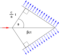
Figure 7: the geometry of Cherenkov radiation. The particle is travelling left to right at speed βc through a medium with refractive index n. The Cherenkov cone has half-angle θ given by cos θ = 1/nβ. In many cases, the particles can be treated as extremely relativistic, β ∼ 1: in this case the opening angle depends only on the medium, cos θ = 1/n. Figure from Wikimedia Commons
An aircraft travelling faster than the speed of sound emits a sonic boom. Similarly, a particle travelling through a transparent medium at faster than the speed of light in that medium emits a kind of “light boom” – a coherent cone of blue light known as Cherenkov radiation. The particle is travelling down the axis of the cone, so if the cone can be reconstructed the direction of the particle can be measured.
Water Cherenkov detectors for neutrinos can be divided into two types:
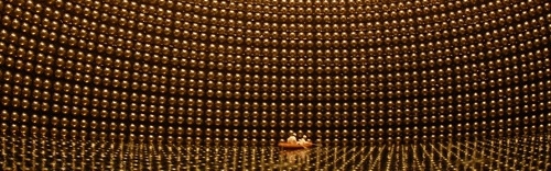
- Densely instrumented artificial tanks (Super-Kamiokande, SNO)
- The water is contained in a tank lined with photomultipler tubes. The Cherenkov light produced by the muon or electron is reconstructed as a ring of hit PMTs. The appearance of the ring can be used to identify the originating particle: muons are single particles, and make sharp rings, whereas electrons (and photons) initiate electromagnetic showers, and the nearly parallel electrons and positrons in the shower combine to make a fuzzy ring. The threshold of these detectors is around 1 MeV or so.
- Sparsely instrumented natural water (neutrino telescopes)
- A very large volume of natural water is instrumented with a sparse array of photomultipliers dispersed throughout the volume (not concentrated at the edges). The cone geometry is not visually apparent, but can be reconstructed using the time at which each hit photomultiplier records its pulse (the opening angle of the cone is known, because these detectors see only high-energy particles). The threshold of these detectors depends on the spacing of the PMTs, but is normally very high (tens or hundreds of GeV); they reconstruct muons, which make a long straight track, much better than electrons, which deposit all their energy in a fairly small volume and are thus seen by fewer PMTs.
Densely instrumented water Cherenkov detectors were foreseen as neutrino detectors by Fred Reines in 1960, but the pioneering IMB and Kamiokande experiments (made famous by their observations of SN 1987A) were originally conceived as detectors for proton decay. At the time, Grand Unified Theories of particle physics predicted that protons should decay (with an extremely long lifetime, of course) into e+ π0. Since the π0 immediately decays into two gamma rays, this is an ideal decay channel for water Cherenkovs, producing an easily recognisable three-ring signature. The protons failed to cooperate – the proton lifetime for this decay channel now stands at >8.2×1033 years – but the experiments proved effective in detecting solar, atmospheric and supernova neutrinos.
Water Cherenkovs can detect the electrons or muons from charged-current interactions, or the recoil electron from neutrino-electron elastic scattering. For solar neutrinos, the latter reaction dominates; for higher-energy neutrinos, the former is more important. Although it might seem that neutrino-electron scattering should be equally sensitive to all types of neutrinos, in fact it is much more sensitive to electron-neutrinos than to other types. This is because electron-neutrinos and electrons can scatter both through neutral-current interactions (the neutrino and electron retain their individual identities, but momentum is transferred from one to the other) and through charged-current interactions (the neutrino converts into an electron, and the electron converts into a neutrino). The presence of this second contribution, which is only possible for electron-neutrinos, greatly increases the chance of interaction. Therefore, water Cherenkovs are essentially electron-neutrino detectors at solar neutrino energies, but detect both electron and muon neutrinos (and flag which is which) at higher energies. (Tau neutrinos are more difficult, for two reasons: because the tau is more massive, the energy threshold above which Cherenkov radiation is emitted is much higher: 0.77 MeV for an electron, 160 MeV for a muon, 2.7 GeV for a tau; also, the tau is extremely short-lived and therefore may not travel far enough to emit much Cherenkov light.) They have good time and energy resolution, and good directional resolution for the detected particle (for low energy neutrinos, this translates into modest angular resolution for the neutrino, because the daughter particle will not be travelling in exactly the same direction as its parent).
Examples of densely instrumented water Cherenkov experiments: Super-Kamiokande (solar neutrinos, atmospheric neutrinos, far detector for K2K and T2K oscillation experiments); IMB (proton decay experiment, 1979–1989, which was one of the two water Cherenkovs to detect neutrinos from SN 1987A).
Examples of neutrino telescopes: IceCube, ANTARES and Baikal.
Heavy-water Cherenkov: SNO
By the mid-1980s, the existence of the solar neutrino problem was becoming established: the theoretical model of the solar interior, the Standard Solar Model of John Bahcall and co-workers, agreed with all observations except the neutrino rate, and all attempts to find a problem with Ray Davis’ experiment had failed. Over the following few years, the deficit of solar neutrinos was confirmed, first by the Kamiokande water Cherenkov experiment and then by the GALLEX and SAGE gallium experiments. It seemed overwhelmingly likely that the source of the problem lay in the behaviour of the neutrino, and specifically in neutrino oscillations. However, there was no “smoking gun”: it could be proven that there was a deficit of electron-neutrinos, but it could not be shown that they had transformed into some other type of neutrino. What was needed was a detector that could directly compare charged and neutral current interaction rates at energies of order 1 MeV, far too low for muon-neutrinos to convert to charged muons.
In 1984, Herb Chen suggested that heavy water might be the solution to the problem. Heavy water, D2O, replaces normal hydrogen by its heavier isotope deuterium (2H or D), whose nucleus contains a neutron in addition to the proton of normal hydrogen. Deuterium is extremely weakly bound, and therefore easily broken up when struck; the key point is that this can happen in two different ways.
- ν + 2H → p + p + e– (charged current), which can only occur for an incoming electron-neutrino;
- ν + 2H → p + n + ν (neutral current), which can happen for any neutrino.
The binding energy of the deuteron is only 2.2 MeV, so any neutrino with an energy greater than this is theoretically capable of initiating the second of these reactions. The two reactions can be distinguished by detecting the capture of the neutron by an atomic nucleus – D2O is not good at capturing neutrons (which is why it’s used as a moderator, to slow neutrons down in nuclear reactors without reducing the flux), but the heavy water can be loaded with some other substance to improve this (SNO used ordinary salt, NaCl; neutrons capture readily on chlorine-35).
Deuterium is a very rare isotope of hydrogen, so heavy water is expensive and difficult to obtain. Fortunately, the Canadian nuclear power industry uses heavy water in its CANDU nuclear reactors, and the SNO Collaboration was able to borrow 1000 tons from Atomic Energy of Canada Ltd. As the loan was for a fixed time, this did place a hard limit on the lifespan of the SNO experiment, which has now concluded; the vessels used to contain the heavy-water active volume and the light-water outer detector (used to reject through-going muons and other background) are being reused by the SNO+ liquid scintillator experiment.
A heavy-water Cherenkov detector is a nearly perfect experiment for low-energy neutrinos, the only drawback being that the threshold is higher than ideal for solar neutrinos (it can see only B-8 and hep neutrinos). The principal disadvantage is simply the unavailability of kilotons of D2O.