The position of neutrinos in the original formulation of the Standard Model can be summarised as follows:
- there are three distinct neutrinos, one for each charged lepton, and three antineutrinos;
- all three neutrinos are massless and left-handed (the antineutrinos are right-handed);
- neutrinos can only convert into their corresponding charged lepton, and vice versa, so that lepton number (the total number of leptons minus the total number of antileptons) is separately conserved for each of the three families, e, μ and τ.
Over the decades since the development of the Standard Model, these properties – which were believed to be well-established – have been seriously undermined. While the rest of the Standard Model has stood essentially unchanged since its first conception, the neutrino sector has had to be conmpletely reconsidered. The driving forces behind this were the Solar Neutrino Problem and the Atmospheric Neutrino Anomaly.
The Solar Neutrino Problem
With hindsight, the first crack in the foundations of the Standard Model picture of neutrinos was already visible before the model was even built. Results from Ray Davis’ chlorine-37 solar neutrino experiment showed that the electron-neutrino flux from the Sun was only about 1/3 of that expected from the predictions of the Standard Solar Model. At the time, this was not taken too seriously by particle physicists, who did not have the technical knowledge to appreciate the reliability of the solar model (there was a tendency for astrophysicists to blame the neutrinos, and particle physicists to blame the astrophysics). However, in the late 1980s the reality of the deficit was confirmed by Kamiokande-II, which observed only 46(±15)% of the expected flux of high-energy solar neutrinos (>9.3 MeV), and a few years later this was joined by the GALLEX and SAGE gallium experiments, which saw about 62(±10)% of the SSM prediction for energies >0.233 MeV. Because elastic scattering preserves some directional information, K-II could demonstrate that its neutrinos really were coming from the Sun; the GALLEX and SAGE experiments calibrated their efficiency using artificial radioactive sources.
Therefore, by the mid-1990s, the Solar Neutrino Problem had become a real issue. The challenges faced by theorists attempting to explain the observations can be summarised as follows:
- All experiments see fewer neutrinos than predicted.
- However, the different experiments see different deficits (see figure 10).
- Different experiments sensitive to the same neutrinos, e.g. GALLEX and SAGE, do agree, suggesting that the differences are likely to be real.
- If the deficit is a function of energy, it isn’t a simple one: water Cherenkovs (high threshold) and gallium experiments (low threshold) both see proportionally more neutrinos than the chlorine experiment (intermediate threshold).
Figure 10: the solar neutrino problem, as of the year 2000. The blue bars are measured values, with the dashed region representing the experimental error; the central coloured bar is the Standard Solar Model with its error. Each colour corresponds to a different type of neutrino, as shown in the legend. Note that because neutrino interaction probabilities depend on energy, the expected number of neutrinos detected from each process is not strictly proportional to the number produced by each process. Figure by John Bahcall.
Any theory seeking to explain the data would have to reproduce these features.
At first, the candidate explanations could be divided into two broad classes: either there’s something wrong with the solar model, or there’s something wrong with the neutrinos.
- There’s something wrong with the solar model.
- The results from the gallium experiments were more-or-less consistent with the idea that the pp neutrinos were being produced at roughly the right rate, but the Be-7 neutrinos were missing. The Be-7 neutrinos come from the pp-II chain (see figure 5), which is more strongly temperature dependent than the pp-I chain – so perhaps the temperature of the Sun’s core has been slightly overestimated, suppressing the pp-II chain. If the Be-7 neutrinos are missing, this would also allow the chlorine and water Cherenkov results to be consistent, in terms of the fraction of the expected flux that is seen.
- The problem with this idea is that, as can be seen from figure 5, boron-8 is made from beryllium-7. There is no way to run the pp-III chain without also running pp-II – and you need pp-III, because there must be some boron-8 neutrinos (or Kamiokande wouldn’t see any signal at all). This argument was supported by the wide range of independently calculated solar models available at the time, all of which predicted that the B-8 and Be-7 neutrino fluxes were tightly correlated.
- There’s something wrong with the neutrinos.
- The initial guess, based on Davis’ results, was that the flavour of the produced neutrinos was somehow randomised between the Sun and the Earth, leading to a reduction of a factor of 3 in the observed flux (because Davis could see only electron-neutrinos). The results from the other experiments showed that this was too simple an idea, since they saw significantly more than 1/3 of their predicted numbers. Obviously, a more complicated solution would be required.
By the mid-1990s, therefore, it appeared unlikely that the Standard Solar Model could be the solution to the Solar Neutrino Problem. The technology required to explain it using neutrino properties, neutrino oscillations, had been invented as long ago as 1957, by Bruno Pontecorvo, and oscillation solutions to the problem had begun appearing in physics journals as early as 1980. However, most of the conventional particle physics community regarded solar neutrinos as an obscure corner of neutrino physics, difficult to understand and probably untrustworthy. Hence, the evidence that was seen as definitively pointing to neutrino oscillations came from another source.
The Atmospheric Neutrino Anomaly
Meanwhile, various experiments across the world were beginning to make measurements of atmospheric neutrinos, initially with a view to determining the background that these would present for proton decay experiments. As discussed above, atmospheric neutrinos are produced by cosmic rays impacting on the Earth’s atmosphere, and should consist of muon-neutrinos and electron-neutrinos in the ratio of 2:1, or perhaps a bit more. However, experiments’ efficiency for detecting and identifying muons is typically different from their efficiency for electrons, so most experiments chose to report their results as a double ratio: (muon:electron)observed/(muon:electron)predicted, where the “predicted” ratio was evaluated after simulating the detector response and passing through the whole experimental analysis chain. If the observations agreed with predictions, this ratio should be 1 within experimental error.
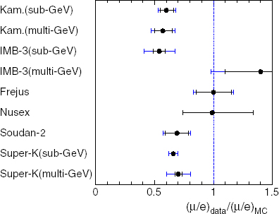
Figure 11: compilation of results on the atmospheric neutrino anomaly, from reference 6.
Though there had been some earlier hints, useful results began to appear in the late 1980s and early 1990s. Initially, these were problematic, as shown in figure 11: water Cherenkov detectors (Kamiokande and IMB) saw anomalously low double ratios, representing a significant deficit in muon-neutrinos, while tracking calorimeters (Fréjus, NUSEX) saw no discrepancy. The coincidence that the results appeared to be correlated with detector type sparked suspicions that some kind of systematic error was involved: fortunately, by 1994 Soudan-2, a tracking calorimeter, was reporting results in line with the water Cherenkovs, lending credibility to the reality of the muon-neutrino deficit.
Figure 12: typical zenith angle distribution, from Super-K. The amount by which the data fall short of the expectation (red line) increases as the distance travelled increases.
In 1998, Super-Kamiokande published detailed studies, using several different sub-samples of data (sub-GeV, multi-GeV, fully-contained, stopping, through-going). A striking feature of these results was the zenith angle distribution for muon-neutrinos, as shown in figure 12: the deficit occurred only in the upward-going sample, where the neutrinos had passed through the Earth before being detected. This is not caused by absorption of the neutrinos within the Earth – the interaction probability for neutrinos of this energy is far too small for that to be a problem, and no such deficit was seen for electron-neutrinos. However, if the neutrinos are oscillating from one flavour to another, the probability that a neutrino created as a muon-neutrino is observed as a muon-neutrino depends on the distance travelled, In this picture, the number of muon-neutrinos was lower for zenith angles >90° because these neutrinos had travelled a greater distance. The distribution predicted using this model, the green line, fits the data very well – as it did for all the subsamples (for example, figure 14 in [6] gives 8 separate muon zenith angle plots, all well fitted by oscillations).
For most members of the particle physics community, the publication of the Super-Kamiokande results marked the “discovery” of neutrino oscillations, despite the long previous history of solar neutrino measurements. The absence of any excess in the electron-neutrino sample indicated that the oscillation being observed was not νμ → νe; Super-K concluded that the best explanation was νμ → ντ, with the tau neutrinos unobserved because of the high mass and short lifetime of the tau lepton.
The Resolution – Neutrino Oscillations
So what are these neutrino oscillations, and how do they work?
The fundamental idea behind oscillations is the quantum-mechanical concept of mixed states, the best-known example being Schrödinger’s infamous cat. In quantum mechanics, if there is a 50% chance that the cat is alive, and a 50% chance that it is dead, then until it is observed it is in a mixture of the two states. For neutrinos, the same idea can lead to oscillation. Although the neutrino is in a well-defined flavour state when it is produced (defined by the charged lepton with which it was associated), and it is in a well-defined flavour state when it interacts, it is not in a well-defined flavour state when it travels between the two. The property that is well-defined as the neutrino travels is its mass: as there are three different types of neutrino, there will be three distinct mass states – but in general these will not line up perfectly with the three different flavour states. The consequence of a mismatch is as follows:
- A neutrino is produced, say in pion decay. It is in a definite flavour state – in this case, it’s a muon-neutrino. It is not, however, in a definite mass state: in fact, it’s a mixture of all three possible mass states in well-defined proportions, say 5% mass 1, 45% mass 2 and 50% mass 3.
- The neutrino travels away from its production point. As it does so, the three mass states get out of step – because they have different masses, they travel at slightly different speeds. Therefore, when the neutrino has gone some distance, the relative proportions of the different mass states will have changed relative to what they were originally. This means that the neutrino is no longer in a definite flavour state, because it’s no longer 5% mass 1, 45% mass 2, and 50% mass 3.
- The neutrino interacts again. Because it is now in a mixed flavour state, there is a certain probability that it will interact as a muon-neutrino, but also a certain probability that it will behave as an electron-neutrino or a tau-neutrino. If our experiment is only set up to detect muon-neutrinos, we will see fewer than we expect.
The mathematics of oscillation is essentially identical to the mathematics of rotation. If only two flavours and two masses are involved, the rotation can be described by a single angle θ – for three flavours, three angles are required, and the mathematics becomes much more complicated.
Figure 13: rotating coordinate axes. The black axes represent the flavour states: the black star marks a neutrino in a pure electron-neutrino state. The red axes, rotated by an angle θ, represent the mass states. Note that the black neutrino is not in a pure mass state: it contains a mixture of both masses. The red star is a neutrino in a pure mass state, but it is a mixture of flavours. When it interacts, it is not certain whether it will do so as an electron-neutrino or a muon-neutrino.
For the two-flavour case, it is fairly simple to work out the probability P that a neutrino produced as flavour α will be observed as flavour β: it is
P(α→β) = sin2(2θ) sin2(1.267 Δm2 L/E)
where θ is the mixing angle, Δm2 is the difference in the squares of the masses, m22 – m12, in (eV)2, L is the distance travelled in km, E is the energy in GeV, and 1.267 is a constant put in to make the units come out right. The important thing to notice about this formula is that θ and Δm2 are properties of the neutrinos, but L and E are properties of the experiment. The important number for a neutrino experiment is therefore the ratio L/E: if your beam energy is twice that of your rivals, you can make the same measurement by putting your detector twice as far away (or, if you already have a detector that is a known distance away, you can design your neutrino beam to make best use of it by adjusting E – this is what we did in T2K).
Solar neutrinos and the MSW effect
The simple two-flavour oscillation worked well to explain the atmospheric neutrino anomaly. The solar neutrino deficit, however, presented more difficulty. The problem is as follows:
- The neutrinos from the Sun don’t all have the same energy, so they don’t all oscillate with the same frequency. If L/E is much greater than 1, so that the neutrinos oscillate back and forth many times on the way from the Sun to the Earth, you would therefore expect the detailed sine-wave structure of the probability to wash out into either 1/2 (if only two neutrino flavours are involved) or 1/3 (if all three are), independent of the exact energy. This clearly isn’t happening: figure 10 shows that neutrinos of slightly different energies have significantly different survival probabilities.
- Therefore we must be seeing the neutrinos after only one or two oscillations, so that different values of L/E produce definitely different results, even if the change in E is quite small.
- But the Earth’s orbit round the Sun isn’t quite circular: we are about 3% closer to the Sun in January than we are in June. If small changes in E cause noticeable changes in the oscillation probability, so should small changes in L – we should see the survival probability change over the course of the year. This doesn’t happen.
The solution to this problem turned out to lie in the fact that solar neutrinos are produced, not in the near-vacuum of the upper atmosphere or a particle accelerator, but in the ultradense matter of the Sun’s core. In this dense material, electron-neutrinos tend to interact with the many free electrons present in the hot, dense plasma deep in the Sun. There aren’t any free muons or taus, so the other neutrinos are not affected. This difference turns out to change the effective parameters of the oscillation, a phenomenon known as the MSW effect after the initials of the three theorists who first worked it out – the Russians Mikheyev and Smirnov, and the American Wolfenstein.
Figure 14: neutrino fluxes from SNO. The x-axis shows electron-neutrino flux, the y-axis flux of other neutrinos (it is not possible to distinguish μ and τ). The red band shows the result of the charged-current analysis, sensitive to electron-neutrinos only; the blue band is the neutral-current analysis, equally sensitive to all types. The green band is elastic νe scattering, which prefers electron-neutrinos but has some sensitivity to other types, and the brown band is the higher-precision result on this from Super-K. The band between the dotted lines is the total neutrino flux expected in the Standard Solar Model.
The key feature of the MSW effect is that under certain conditions it is resonant – it efficiently converts (nearly) all electron-neutrinos into some other type. For the Sun, the low-energy neutrinos produced in the pp reaction are almost unaffected, whereas higher energy neutrinos hit the resonance: this accounts for the apparent near-total disappearance of the Be-7 neutrinos. A feature of the resonance is that it only happens if the mass state that is mostly electron-neutrino is lighter (in a vacuum) than the one it transforms into – thus we know that the mostly-electron-neutrino mass state is not the heaviest of the three. In contrast, “ordinary” oscillations, taking place in a vacuum, don’t tell us which of the two states is heavier.
This explanation of the solar neutrino deficit was dramatically confirmed a few years later by the SNO heavy-water experiment, which used dissociation of deuterium to compare charged-current and neutral-current neutrino interaction rates directly. As seen in Figure 14, their results clearly show that the “missing” solar neutrinos are not missing at all: they have simply transformed into some other type. This is definitive evidence in favour of neutrino oscillations.
Neutrino Masses
The probability that neutrino type α transforms into type β is zero if Δm2 = 0: if neutrinos were massless, or indeed if they all had the same mass, they could not oscillate. This is because, however you label the neutrinos, the total number of distinguishable types must remain the same, i.e. three. If there aren’t three different masses, mass isn’t a valid labelling scheme, so the neutrinos’ identities must be defined by their interactions and there is no oscillation. This is very like locating a place on a map: you can use longitude and latitude, or Ordnance Survey map references, or a distance and bearing from a reference point (“5 km northeast of the railway station”), but you always need two numbers (three, if you also want to specify height above sea level).
Figure 15: Δm2 and θ for the solar neutrino oscillation. This is the best combined fit to the solar neutrino data and the KamLAND reactor neutrino data, from reference 7.
By counting the number of neutrinos they observe, experimenters can find values for the unknown Δm2 and θ in the equation for the survival probability (L and E are known from the design of the experiment). Recent results for the solar neutrino and atmospheric neutrino oscillations are shown in figures 15 and 16. Clearly the parameters are not the same, but this is to be expected: in the case of solar neutrinos we start with νe and end with something else, whereas for atmospheric neutrinos we start with νμ and end with ντ, so we are looking at different systems. It is usual to call the solar neutrino mixing θ12 and the atmospheric mixing θ23.
Because the oscillation is only sensitive to the difference in the squared masses, these results tell us that the masses are not zero, but don’t tell us what they are. The squared mass difference of 8×10⁻⁵ eV2 between mass 1 and mass 2 could correspond to 0 and 0.009 eV, 0.01 and 0.0134 eV, 0.1 and 0.1004 eV, or even 10 and 10.000004 eV – the oscillation results do not tell us. For the atmospheric neutrinos, we don’t even know which state is heavier. This gives us two possible ways to combine the two values of Δm2:
Normal Hierarchy: ν1 ← 8×10⁻⁵ → ν2 ← 2.3×10⁻³ → ν3;
Inverted Hierarchy: ν3 ← 2.3×10⁻³ → ν1 ← 8×10⁻⁵ → ν2.
Figure 16: Δm2 and θ for the atmospheric neutrino oscillation. This plot shows both atmospheric neutrino data from Super-Kamiokande and accelerator neutrino data from MINOS, from reference 8.
We know from the solar data that mass state 1 is mostly electron-neutrino, so the “normal hierarchy” is so called because it assumes that the lightest neutrino corresponds to the lightest charged lepton. Figure 16 shows that the mixing between νμ and ντ is pretty much as large as it could possibly be (θ23 ∼ 45°), so it doesn’t really make sense to assign mass states 2 and 3 to “μ” and “τ” – they contain equal amounts of each.
Measuring the neutrino mass using beta decay
The next generation of neutrino oscillation experiments should be able to work out the ordering of the mass states, and will improve the precision with which we know the mass splittings. To measure the masses themselves, we need to go back to the original inspiration for the idea of the neutrino – beta decay.
In beta decay, the available energy (the difference between the masses of the radioactive parent nucleus and its daughter) is shared between the electron and the neutrino. The electron, however, must get at least mec2, because its energy must be at least enough to create its own mass. If the neutrino had exactly zero mass, it could be very unlucky and get zero energy. However, we now know that neutrinos are not massless, so we have to allow the neutrino to carry away at least mνc2. This slightly reduces the maximum possible energy that could be given to the electron, so the distribution of electron energies will be modified slightly near its endpoint.
Unfortunately, it is very unlikely that the energy split between the electron and the neutrino should be so one-sided, so regardless of the isotope we choose, the number of decays in this region of the electron energy spectrum will be very small. Furthermore, because we expect that the neutrino mass is extremely small, we will need to measure the electron energy with very high precision: a small experimental uncertainty could easily wipe out our signal. Electrons are charged, so their energy is affected by electric fields – the eV unit of energy is just the energy an electron gains from a voltage drop of one volt – so if our experiment uses electric fields we need to be very careful to ensure that they do not affect the electron energies we are trying to measure. If the isotope in the experiment is in the form of a chemical compound, even the electric fields associated with the chemical bonds may be enough to distort the results, and will need to be calculated and corrected for. In short, this is a very difficult experimental measurement, and it is not surprising that nuclear physicists have been working on it for years without success (in the sense that they have failed to detect any difference from the expectation for zero mass).
The best limits on neutrino mass from beta decay come from the decay of tritium, 3H or T, which decays to helium-3 with a half-life of 12.3 years. Tritium is a good isotope to study because:
- the mass difference between 3H and 3He is rather small, only 18.6 keV (0.00002 atomic mass units) – this makes the small distortion of the spectrum caused by a non-zero neutrino mass more visible;
- the half-life is comparatively short, which means you don’t need a large amount of tritium to generate a large sample of decays;
- tritium is a very simple atom, and its natural molecular form T2 is a very simple molecule – this makes calculating the effects of the molecule’s internal fields on the electron energy fairly simple.
The combination of small mass difference and short half-life is very unusual – normally, if the mass difference is very small, the half-life is very long, because the atom doesn’t “gain” much by decaying. For example, the isotope rhenium-187 has an even lower maximum energy release – only 2.6 keV – but its half-life is 43 billion years! Therefore, over the years since this experiment was first tried in the 1940s, tritium has been the isotope of choice in almost every case.
The current state of the art in tritium beta decay is the KATRIN experiment at Karlsruhe. The key to an accurate mass measurement is high-precision measurement of the electron kinetic energy, which KATRIN achieves using a so-called MAC-E filter (short for Magnetic Adiabatic Collimation with Electrostatic filter). KATRIN’s current upper limit is 1.0 eV (i.e. their data are consistent with zero mass; they would have seen a signal for a mass above 1.0 eV), but this is based on only a month’s run time, and their eventual goal is around 0.2 eV.
In addition, the low-energy but long-lived isotope 163Ho is the basis of the HOLMES experiment. 163Ho decays by electron capture with a half-life of 4570 years and an energy release of 2.883 keV. HOLMES uses a calorimetric technique in which the holmium is embedded in cryogenic “microcalorimeters” – essentially very sensitive thermometers – which will measure all the energy released in the decay except for that carried off by the neutrino. As with the tritium experiments, the aim is to measure the end-point of the energy spectrum to look for a cut-off corresponding to a non-zero neutrino mass.
Although the holmium technology is less mature than the tritium experiments, and the expected sensitivity is less than that of KATRIN, it is important to have two different experiments using very different techniques attacking this difficult problem. We saw above that the solar neutrino deficit was only really taken seriously when it was confirmed by a second experiment: the field of neutrino physics has a history of false alarms which has made the community conservative in its approach to new results. Although the first experiment to report a non-zero result will eventually get the credit, recognition may well have to await confirmation by a second team.
Majorana neutrinos and neutrinoless double beta decay
The Standard Model picture of neutrinos assumes that, as with all the other quarks and leptons, the neutrino and the antineutrino are quite distinct particles. In the other cases, this can be confirmed by their electric charges: the electron has negative charge, its antiparticle the positron has positive charge. Even in the case of the neutron, which is neutral overall, the quarks composing it have different charges (+2/3 –1/3 –1/3 for the neutron, –2/3 +1/3 +1/3 for the antineutron), and this can be confirmed by scattering experiments. Of the matter particles, as opposed to the force carriers, only the neutrino is both neutral and (as far as we know) genuinely elementary. This introduces a possible alternative to the concept of separate neutrinos and antineutrinos: what is the two particles were in fact identical, but only their spin direction differed? Because of the structure of the weak interaction, left-handed neutrinos would only interact as neutrinos, while right-handed neutrinos would interact as if they were antineutrinos. As long as their handedness remained unchanged, the two would behave as entirely different particles, even though in principle they were not.
A neutrino which behaves like this is called a Majorana neutrino, after the Italian theorist Ettore Majorana who first worked out the relevant mathematical description. If the neutrino were precisely massless, its handedness would be fixed, and there would be no meaningful distinction between the two pictures: all neutrinos would be left-handed, always, and all antineutrinos would be right-handed. But oscillations tell us that neutrinos cannot be exactly massless, and if they are not, then their handedness is not an unchangeable constant. Therefore, if neutrinos really are Majorana particles, it is possible in principle (if very improbable in practice, because their masses are so small), that a particle produced as a neutrino might be capable of subsequently interacting as an antineutrino. This behaviour might be seen in a very rare kind of radioactive decay called double beta decay.
Ordinary beta decay takes place when an atom converts a neutron to a proton (emitting an electron and increasing its atomic number by 1) or a proton to a neutron (emitting a positron and decreasing its atomic number by 1). This happens when the neighbouring isobar (atomic nuclei with the same atomic mass, i.e. the same total number of protons and neutrons, are called isobars) is more tightly bound, and hence has less mass, than the one that beta-decays. Howver, in some circumstances, although both neighbouring isobars weigh more than the atom in question, one of the isobars two units away in Z weighs less. In this case, the only permitted mode of decay is double beta decay, in which the nucleus simultaneously emits two electrons (and, in the Standard Model, two neutrinos – a process known as 2νββ). This is a very improbable event, and hence the lifetimes of such isobars are much, much longer than the age of the universe – at least 1019 years. For most purposes, isotopes which can only decay by double beta decay can be regarded as stable: indeed, of the 60 or so nuclear species which could in principle decay in this way, only 11 have been observed to do so.
2νββ decay is completely consistent with the original Standard Model massless neutrinos. However, if the neutrino is a Majorana particle, a modified form of this decay is possible, in which the particle emitted as a neutrino by one of the beta decays is absorbed, as an antineutrino, by the other, producing neutrinoless double beta decay (0νββ) as in figure 17.
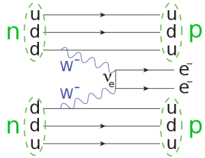
Figure 17: double beta decay. Two neutrons are converted to two protons, with the emission of two electrons. The neutrino emitted by one of the decays is absorbed, as an antineutrino, by the other. Figure from Wikimedia Commons.
Double beta decay violates lepton number conservation by 2: two electrons are produced with no corresponding antileptons. It is only possible if neutrinos are Majorana particles, so its discovery would establish the nature of the neutrino as well as a value for the mass (as we are producing electrons, the neutrino in the diagram is an electron-neutrino, so it is not a well-defined mass state: the mass we measure is a weighted average of the three possible values).
The signature of 0νββ decay is two electrons produced back-to-back, each with the same energy (corresponding to half the mass difference between the parent and daughter nuclei). In contrast, in 2νββ decay the electrons come out with a continuous energy spectrum, similar to figure 1 (in which the red line would represent the 0νββ signal). All 0νββ isotopes do of course also decay by 2νββ, so the key to a successful measurement is the ability to detect a small peak at the endpoint. And it is a small peak: lifetimes for 0νββ decay are at least 1025 years – a million times longer than the 2νββ mode.
The key requirement for a 0νββ experiment is to minimise background, since the signal is so small that even a small amount of background near the expected peak position has a serious effect on your sensitivity. The potential backgrounds include:
- natural radioactivity, in your source itself (as a result of impurities), your detector, or the surrounding environment – minimising this requires the use of ultrapure materials in the experiment itself and good shielding from the environment;
- cosmic rays and cosmogenic radioactivity – therefore experiments are normally located, and ideally manufactured, underground;
- the 2νββ mode – unavoidable, but distinguishable from the 0νββ signal by the energy of the electrons and their back-to-back topology.
There are two basic techniques used in double beta decay experiments: source = detector (the isotope being measured is, or forms part of, the detector used to measure the decay) and passive source (the isotope is not part of the detector). The former type are usually cryogenic solid-state detectors measuring the ionisation produced by the decay electrons. They have good energy resolution, which is important for background suppression, and are quite small, which makes them easier to shield from environmental radioactivity. Most experiments also use the shape of the signal pulse to discriminate against background: neutrons from cosmic rays look different from electrons.
In passive-source experiments, the radioisotope is in the form of a thin film, surrounded by detector elements. These experiments usually have significantly poorer energy resolution, but can use the back-to-back topology of the emitted electrons to reduce background, since they have tracking capabilities (which the source = detector experiments generally don’t). They have the advantage that they can investigate many different isotopes with the same detector (sometimes at the same time).
The double-beta decay isotope 136Xe is a special case, being a noble gas rather than a solid. It can be used, in gaseous or liquid form, as the medium for a tracking detector, similar to those used in passive-source experiments; it is also a popular candidate for ton-scale dark-matter experiments, some of which could in principle double as double-beta experiments. Unfortunately, the double-beta isotope is a relatively minor constituent (8.86%) of natural xenon, so to optimise performance the xenon has to be expensively enriched.
Most double-beta decay experiments have measured the 2νββ decay and set limits on the 0νββ decay. There is a controversial claim of a positive detection of 0νββ decay of 76Ge from the Heidelberg-Moscow experiment, corresponding to a mass of 0.4 eV (with a factor 2 uncertainty from theoretical uncertainties in the nuclear physics calculations [the nuclear matrix element]). This result is disputed, largely because there are several peaks in the endpoint region, and critics are not convinced that the one that matches the endpoint energy is not just another one of these. The GERDA experiment, using the same isotope but with higher mass and greater sensitivity, was designed to confirm or refute this disputed claim. GERDA presented its final results in 2020, observing no signal and setting a limit on the 0νββ decay of 76Ge of 1.8×1026 years (compare this with the age of the universe, a mere 1.4×10¹⁰ years!). This corresponds to a neutrino mass limit of about 0.1 to 0.2 eV (the number is not exact because of theoretical uncertainties), but of course this is only valid if neutrinos are indeed Majorana particles.
Several neutrinoless double beta decay experiments are currently operating, commissioning or under construction, all with planned sensitivities at the 0.1 eV level or better (see the Wikipedia article for a list of links). The experiments cover a wide range of isotopes, which is a good thing: the theoretical calculations of the nuclear matrix elements, necessary to predict the decay rates and to interpret any signal in terms of its implications for the neutrino mass, have large errors, and comparisons of signals from different isotopes would surely help to alleviate this. Although it seems to be easier to achieve this sensitivity in neutrinoless double beta decay than in single beta decay, we should remember that the tritium and rhenium beta-decay experiments will work for any type of neutrino, whereas the double-beta decay experiments require a Majorana neutrino.
Neutrino masses from astrophysics and cosmology
Neutrinos are extremely common in the universe: stars make them in vast numbers, and they were even more copiously produced in the first few seconds of the Big Bang. It was once thought that neutrinos with masses of order 10 eV or so might account for the dark matter, until simulations of the formation of structure in the universe showed that such fast-moving particles would produce the wrong kind of large-scale structure, making very large objects – galaxy superclusters – first, and smaller objects – galaxies – rather later (top-down structure formation). The universe we see is more consistent with a history in which galaxy-sized structures formed fast and later collected into larger systems (bottom-up structure formation), which implies fairly slow-moving, probably more massive, dark-matter particles.
However, because there are so many of them (on average, 336 per cubic centimetre everywhere in the universe, according to calculations), even the much lighter neutrinos that we currently imagine, with masses of order 0.1 eV, would contribute something to the density of the universe. This might be detected through its effect on the spectrum of temperature variations in the cosmic microwave background, as measured by WMAP and Planck. The 2015 analysis of the Planck data sample[9]] quotes a limit ∑ mν < 0.23 eV from a combined analysis of the cosmic microwave background and galaxy redshift surveys. Taken at face value, this is the most stringent limit on neutrino masses currently available; it does, however, make some assumptions about the underlying cosmological model (specifically, that it has a flat geometry, and that the dark energy can be described as a cosmological constant). These are not guaranteed to hold, and therefore the quoted limit is not bullet-proof.
Supernova 1987A was also used to set neutrino mass limits. If the neutrino were massless, all neutrinos would travel at exactly the speed of light: since neutrinos aren’t exactly massless, they travel more slowly than light, and their speed depends on their energy (more energetic neutrinos travel more quickly). Therefore, one would expect the more energetic neutrinos from SN 1987A to arrive here sooner than the less energetic ones, so the time distribution of the incoming neutrinos can be used to infer their masses.
This would work very well if the neutrino pulse from a supernova were instantaneous. Unfortunately, as can be seen from figure 7, it isn’t, so the intrinsic time profile of the neutrino emission has to be taken into account; furthermore, the mean energy of the neutinos also evolves with time as the explosion progresses. With a large sample of neutrinos, these effects might be disentangled: with the 20 or so from SN 1987A (not all of which could safely be compared, since the Kamiokande-II and IMB clocks were not synchronised), this is not really possible, and the limits obtained were not competitive.